
The density-bounded sina plot offers a sophisticated alternative to standard jittering by constraining individual data points within their calculated kernel density envelopes. This fundamental advancement in the grammar of graphics allows researchers to move beyond the limitations of base ggplot2, which often struggles to represent high-dimensional data without overplotting or losing critical distributional details. The ggforce package, meticulously developed by Thomas Lin Pedersen, serves as a powerful extension that bridges the gap between general exploratory visualization and publication-grade scientific illustration. By integrating seamlessly with the existing ggplot2 ecosystem, it introduces specialized geoms, stats, and coordinate transformations that empower users to communicate complex experimental findings with precision. This tool has become indispensable for those working in data-heavy fields, providing a bridge between raw statistical output and intuitive visual storytelling that adheres to the rigorous standards of modern academic and industrial reporting.
1. Applications: Scientific Data Communication
In quantitative empirical research, communicating complex experimental distributions, clustering patterns, and multiscale observations often exceeds the default graphical vocabulary of base ggplot2. While ggplot2 excels at general exploratory data investigation, core design decisions intentionally omitted specialized geometric primitives to prevent API bloat and maintain a streamlined user experience. The ggforce package addresses these specific gaps by implementing a wide array of specialized stats, geoms, and facets that adhere strictly to ggplot2 extension conventions. Investigators across diverse disciplines—including bioinformatics, computational biology, oncology, and economics—increasingly rely on these tools to solve visualization bottlenecks that occur when datasets grow in both size and complexity. By providing a structured way to handle these challenges, the package ensures that the underlying story of the data is not lost in a sea of standard, and sometimes inadequate, default plotting options.
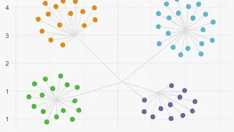
When analyzing high-dimensional single-cell RNA sequencing or flow cytometry embeddings, standard scatter plots frequently obscure dense groupings and cluster boundaries due to the sheer volume of overlapping points. Using the specialized annotation tools within ggforce, researchers can automatically compute and draw concave hulls around phenotypic subpopulations, providing clear visual boundaries accompanied by descriptive callout labels. In clinical trial cohorts and pharmacokinetic studies where sample sizes across treatment arms vary widely, traditional boxplots or violin plots can inadvertently mislead readers regarding observation density. This package resolves such issues through density-controlled point dispersion, ensuring that the visual weight of the data accurately reflects the underlying sample sizes. This precision is vital for maintaining scientific integrity, especially when data distributions are non-normal or contain significant outliers that demand closer inspection.
2. Setup: Technical Prerequisites and Installation
The ggforce package is actively maintained on the Comprehensive R Archive Network (CRAN) under the permissive open-source MIT license, making it a reliable choice for long-term projects. Because the package incorporates compiled C++ code through the modern cpp11 interface and interfaces with underlying geometric libraries such as polyclip, a system must meet standard development prerequisites before a successful installation can occur. Currently, the package requires R version 3.3.0 or higher and ggplot2 version 3.5.0 or higher to function correctly. For users operating on macOS systems, it is essential to ensure that Xcode Command Line Tools are installed, while Windows users should install the version of Rtools that matches their specific R installation. On Linux distributions, ensuring that standard C++ compilation packages, such as build-essential on Ubuntu or Debian, are installed will prevent common errors during the build process.
To install the current stable release directly from the official CRAN repository, the standard installation command should be executed within an active R console. While the core package imports fundamental tidyverse infrastructure—including rlang, scales, gtable, and vctrs—several of its more advanced geoms rely on optional companion libraries to unlock their full analytical potential. To avoid runtime warnings and access features like concave hulls or physical unit scaling, researchers are encouraged to install a suite of recommended libraries including concaveman, deldir, and units. Once these components are in place, verifying the installation by loading the libraries and querying the runtime version ensures that the environment is ready for high-stakes visualization tasks. This systematic approach to setup minimizes technical debt and ensures that the visual output remains consistent across different computing environments and collaborative laboratory clusters.
3. Distributions: Implementing Sina Plots and Convex Hulls to Facilitate the Visualization of Large Datasets
The initial step in creating advanced visualizations involves loading the necessary libraries and preparing the experimental dataset for processing. In this demonstration, the standard Iris dataset is utilized to represent recorded dimensions across various species as a proxy for the complex treatment arms found in clinical research. Constructing a density-bounded Sina plot through the geom_sina() function offers a significant improvement over standard jittering techniques. Unlike random noise applications, this method constrains point displacement strictly within the kernel density envelope of each group, ensuring that the visual representation of data points remains faithful to the actual distribution. By setting parameters like ‘scale’ to ‘area’ and ‘method’ to ‘density,’ the user ensures that the total area of the jitter envelope is proportional to the number of observations, preventing the overlapping of points with adjacent categorical axis ticks and maintaining a clean, professional aesthetic.
Highlighting specific phenotypic clusters requires a more organic approach than simple rectangles or circles, leading to the use of concave hulls. By invoking geom_mark_hull(), researchers can trace an organic perimeter around designated groupings, utilizing the concaveman algorithm to calculate boundaries that hug the data points without including large, vacant spaces. This function also automates the placement of non-overlapping callout labels, which include both titles and descriptive narrative text, thereby eliminating the need for tedious manual post-processing in external vector illustration software. Adjusting the concavity parameter allows for fine-tuned control over how tightly the hull indentations follow the data cloud, while expansion and radius parameters provide necessary padding and rounding. This level of automation is essential for high-throughput data pipelines where hundreds of individual plots must be generated and annotated with consistent geometric rules.
4. Detail: Advanced Faceting and Magnification
When investigating dense clusters or identifying subtle microstructures within a larger dataset, the facet_zoom() function provides a powerful method for constructing context-preserving magnified views. This feature splits the rendering area into a global overview panel and a detail-oriented magnified panel, allowing the reader to observe specific subgroups—such as a single species or a targeted response zone—without losing sight of the broader data landscape. Visual reference brackets connect the zoom window to the parent dataset, guiding the viewer’s eye between the two scales of observation. This is particularly useful in exploratory analysis where a specific outlier cluster or a congested interval requires closer inspection. By defining a simple logical expression for the focus area, the user can automate the magnification process, ensuring that the detail panel remains synchronized with the primary data layer even as the underlying information is updated or filtered.
As datasets grow to include hundreds of variables or longitudinal observations, standard faceting methods often result in unreadable thumbnails that are unsuitable for formal reporting. The facet_wrap_paginate() and facet_grid_paginate() functions resolve this issue by enabling multi-page document generation directly from the R console. This functionality allows for the division of complex, faceted graphics across a predetermined number of pages or slides, maintaining the legibility of each individual panel. By calculating the total number of required pages with the n_pages() helper function, researchers can automate the export of high-resolution PDF reports through simple iterative loops. This automated approach is particularly valuable for large-scale, multi-subject studies where manual plot arrangement would be prohibitively time-consuming. The resulting multi-page documents provide a clear, uncompressed view of the data that is ready for peer-reviewed submission or internal stakeholder presentations.
5. Interpolation: Trajectories and Parallel Sets
The visualization of continuous transitions and relational paths is another area where ggforce excels, offering specialized geoms for rendering smooth interpolation curves and network trajectories. Functions such as geom_bspline(), geom_bezier(), and geom_link() allow for the creation of mathematical curves that represent cellular differentiation paths, phylogenetic trajectories, or kinetic reaction curves with high precision. These tools provide a grammar-aligned way to draw directional transitions and parameter gradients, moving beyond the simple straight lines that often oversimplify complex biological or physical processes. By adjusting the interpolation granularity, users can balance visual smoothness with computational efficiency, ensuring that the resulting vector graphics remain manageable in size while providing the necessary level of detail for print resolution. This capability is critical for researchers who need to visualize the flow of time or state changes within dynamic experimental systems.
Categorical flow diagrams represent another sophisticated visualization technique supported by the package through the use of parallel sets. The geom_parallel_sets() function serves as a robust alternative to standalone alluvial or Sankey diagrams, enabling the visualization of transitions and multi-attribute contingency tables within the familiar ggplot2 framework. Visual ribbons represent categorical frequencies across sequential dimensions, where the width of each ribbon corresponds to the proportion of observations sharing a specific combination of attributes. Tracking these ribbons across various axes allows researchers to observe how subgroups partition or coalesce throughout a process, such as patient progression through clinical triage and treatment. This integrated approach to flow visualization ensures that categorical transitions are treated with the same statistical rigor as continuous variables, providing a unified visual language for analyzing complex multi-stage experimental workflows.
6. Interpretation: Decoding Complex Geometric Outputs
Interpreting the graphical outputs generated by these advanced functions requires a fundamental understanding of the statistical transformations and geometric algorithms operating behind each visual layer. When reading a Sina plot, the observer must focus on the lateral spread of individual points, as the width of the point cloud at any vertical value corresponds directly to the kernel density estimate. This differs from standard jittering, where the width is arbitrary and uniform. If a subpopulation exhibits a bimodal distribution, the points will form two distinct lateral bulges, providing an immediate visual cue that a simple boxplot would miss. Because every observation is rendered as a discrete glyph, the reader can gauge both the sample size and the distributional density simultaneously, spotting sparse outliers that might otherwise be masked by the smoothed contours of a conventional violin plot or the summary statistics of a mean and error bar plot.
For cluster markings produced by concave hulls or ellipses, the output contains three coordinated components that must be read in tandem: the enclosing boundary, the anchor line, and the descriptive text box. The boundary polygon indicates the spatial extent of a group, with concave hulls providing a more accurate representation of the data’s geometry by avoiding empty intermediate spaces. Callout lines are designed to find the shortest non-conflicting path from the cluster’s center to an open region on the canvas, ensuring that the text remains legible without obscuring the data itself. Similarly, when inspecting zoom facets, the interconnectivity between the overview and the detail panel is key to an accurate interpretation. The tinted rectangular box on the overview panel demarcates the magnified coordinates, allowing the reader to verify local microstructures without losing their spatial orientation relative to the global data domain. This dual-layered approach fosters a more comprehensive understanding of multiscale datasets.
7. Optimization: Troubleshooting and Technical Support
When deploying these tools in automated research pipelines, investigators may encounter technical challenges ranging from missing dependencies to rendering lags. A frequent issue involves missing companion packages like concaveman or deldir, which are often listed as suggested dependencies to keep the initial installation footprint small. If a rendering error occurs, installing these specific packages from CRAN typically resolves the problem. For Linux users, it is important to remember that certain packages interface with the V8 JavaScript engine, requiring the installation of system-level development headers. Another common hurdle is the clipping of descriptive labels at the edges of the plot canvas. This can be mitigated by disabling coordinate clipping and expanding the plot margins, ensuring the automated callout system has enough room to position text boxes near the perimeter of the graphic without truncating the information.
Performance optimization is equally important, especially when dealing with high-density datasets that utilize complex curves or thousands of points. For instance, using smooth interpolation functions like geom_bspline() on massive tables can lead to significant memory overhead and slow PDF compilation times. This occurs because the default settings generate a high number of intermediate coordinates per segment to achieve a smooth appearance. By reducing the interpolation granularity to a lower value, researchers can produce visual smoothing that remains indistinguishable at print resolution while significantly reducing the computational vertex count. Additionally, scale distortion in zoom facets can often be traced back to missing values in filtering variables. Ensuring that data columns are cleaned of NA values before plotting prevents bounding box limits from failing to resolve, resulting in more stable and predictable visual outputs across different subsets of the data.
8. Alternatives: Comparative Visualization Frameworks
The R ecosystem offers several other packages that extend the functionality of ggplot2, each with a specific focus that may complement or overlap with the features found in the current package. For example, ggbeeswarm provides categorical point jittering using density distribution algorithms like quasi-random plots, which are excellent for smaller datasets where point-packing is desired. On the other hand, the ggdist package is specifically tailored for visualizing distributions and statistical uncertainty, making it a preferred choice for communicating Bayesian posterior distributions or confidence intervals through “raincloud” or “half-eye” plots. Understanding these functional divisions allows researchers to select the most appropriate tool for their specific needs, whether they are focusing on point-level detail, cluster annotation, or the clear communication of statistical uncertainty within a complex multi-panel figure.
While some packages specialize in distributional plots, others like ggh4x and ggrepel focus on layout and labeling. The ggh4x package provides extended faceting utilities, such as nested facet headers and custom axis guides, which are invaluable for complex experimental designs with multiple hierarchical levels. Meanwhile, ggrepel remains the industry standard for preventing label collisions on dense scatter plots through a repulsive positioning algorithm. It is also important to note that certain older packages, such as ggalt, have been archived or replaced by more modern implementations like those found in ggforce. By combining these different extensions—using patchwork for multi-plot arrangement and theme customization for aesthetic consistency—researchers can build a comprehensive and robust visualization workflow that meets the highest standards of clarity and technical accuracy in modern scientific publishing.
9. Strategy: Implementation and Next Steps
The successful integration of the ggforce package into a professional research workflow relied on a clear understanding of its geometric logic and technical requirements. Throughout the development of these visualization scripts, the focus remained on enhancing the readability and precision of data representation. Researchers transitioned from standard exploratory plots to complex, publication-ready figures by leveraging sina plots for distribution analysis and concave hulls for cluster identification. This shift ensured that the nuances of high-dimensional datasets were preserved and effectively communicated to external audiences. The automation of multi-page reporting further streamlined the process, allowing for the consistent generation of high-quality outputs even as experimental scales increased.
Moving forward, the primary objective should be the optimization of these graphical pipelines to handle increasingly large datasets without compromising performance. Researchers might consider exploring the use of precomputed coordinate systems or reduced interpolation settings to maintain speed during high-throughput analysis. Additionally, standardizing the use of unit-aware scales will prevent common errors in physical data interpretation and enhance the reproducibility of visual results. By consistently applying these advanced techniques and staying informed about updates in the ggplot2 ecosystem, the scientific community can continue to produce visual evidence that is both mathematically rigorous and aesthetically compelling. This proactive approach to data visualization will ultimately lead to clearer insights and more effective dissemination of complex research findings.