
In the rapidly evolving field of time series forecasting, crafting efficient and adaptable workflows is essential for tackling complex datasets and achieving accurate predictions. GluonTS, a powerful open-source library for time series modeling, offers a robust framework to streamline this process by enabling the integration of multiple models within a single pipeline. This article dives into a practical approach to harnessing GluonTS, focusing on generating synthetic datasets, preparing data for analysis, and running diverse estimators in parallel. By incorporating evaluation metrics and advanced visualizations, a seamless process emerges that not only trains and compares models but also provides clear insights into their performance. This guide aims to equip readers with the tools and knowledge to build flexible workflows that can adapt to various environments and challenges, ensuring actionable results even when dependencies are missing. The step-by-step methodology outlined here serves as a foundation for experimentation, whether working with synthetic or real-world data, making it easier to navigate the intricacies of forecasting with confidence.
1. Setting Up Essential Libraries and Dependencies
Getting started with GluonTS requires a solid foundation of libraries and tools to handle data manipulation, visualization, and model implementation effectively. Key libraries such as NumPy and Pandas are indispensable for managing and processing data, while Matplotlib facilitates the creation of insightful visual representations of results. Additionally, GluonTS utilities provide the necessary components to build and evaluate time series models. A critical aspect of setting up the environment involves conditional imports for backend estimators like PyTorch and MXNet. This approach ensures that the workflow remains flexible, allowing the system to utilize whichever backend is available without crashing due to missing dependencies. By structuring the imports to handle potential errors gracefully, the pipeline can adapt to different setups, whether on a local machine or a cloud-based platform, ensuring that the process continues smoothly.
Beyond the basic setup, attention to dependency management plays a vital role in maintaining workflow stability. For instance, checking the availability of PyTorch and MXNet estimators at the outset helps in planning which models can be included in the analysis. If a particular backend fails to load, the system can fall back to alternative options or built-in datasets, preventing interruptions. This adaptability is crucial in real-world scenarios where software environments may vary widely. Moreover, suppressing unnecessary warnings during execution keeps the output clean and focused on essential information, enhancing readability and usability. This preparatory step lays the groundwork for subsequent tasks, ensuring that the technical environment supports the complex operations of multi-model forecasting without unnecessary hurdles.
2. Generating a Synthetic Multi-Series Dataset
Creating a synthetic dataset serves as an excellent starting point for experimenting with GluonTS, particularly when real-world data is unavailable or too complex for initial testing. The process involves designing multiple time series that incorporate realistic elements such as trends, seasonality, and random noise. By carefully constructing these components, the dataset mimics the challenges often encountered in practical forecasting scenarios, providing a controlled environment to test models. A key feature of this step is ensuring reproducibility, which means setting a random seed so that every run produces consistent results. This consistency is vital for debugging and comparing model performance across different experiments, as it eliminates variability in the data itself.
Once generated, the synthetic data is formatted into a clean, multi-series DataFrame, ready for further processing. This structure allows for easy manipulation and integration into the GluonTS framework, where each series represents a unique entity with its own temporal patterns. Typically, a dataset might include a predefined number of series, such as 10, each spanning a specific length, like 200 time steps. The inclusion of diverse characteristics within the data ensures that models are tested under varied conditions, enhancing the robustness of the workflow. This step not only facilitates hands-on learning but also builds confidence in handling more intricate datasets later, as the principles of data generation can be adapted to suit specific needs or domains.
3. Preparing Data and Splitting for Training and Testing
With a synthetic dataset in hand, the next crucial task is to prepare it for modeling by converting it into a format compatible with GluonTS. Using the PandasDataset class, the multi-series data is structured to align with the library’s requirements, specifying the target columns for forecasting. This conversion ensures that the data can be seamlessly fed into the models for training and evaluation. A typical setup might involve a dataset with 10 series, each containing 200 time steps, and a prediction length of 30 days. This preparation phase is essential for aligning the data structure with the expected input format of various estimators, minimizing errors during model execution.
Following preparation, the dataset must be split into training and testing segments to facilitate accurate model assessment. This split is often achieved by defining an offset, such as the last 60 time steps, to separate historical data for training from future data for testing. Additionally, test instances are generated with specific windows to evaluate model performance over multiple forecasting horizons. This methodical division ensures that models are trained on past patterns while being tested on unseen data, mirroring real-world forecasting challenges. Proper splitting and preparation are pivotal in establishing a reliable evaluation framework, allowing for meaningful comparisons across different models and configurations within the GluonTS environment.
4. Initializing Multiple Forecasting Models
The strength of GluonTS lies in its ability to support multiple forecasting models within a unified pipeline, catering to diverse analytical needs. This step focuses on initializing various estimators, such as PyTorch DeepAR, MXNet DeepAR, and SimpleFeedForward, provided the respective backends are available in the environment. Each model is configured with specific parameters, like frequency set to daily and a prediction length of 30 time steps, to align with the dataset’s characteristics. This initialization process is designed to be robust, incorporating error handling to manage situations where certain backends might fail to load due to missing dependencies or compatibility issues.
To ensure an uninterrupted workflow, a fallback mechanism is implemented. If no external backends are accessible, GluonTS can resort to a built-in artificial dataset with predefined seasonal patterns. This contingency plan allows the pipeline to proceed with model training and evaluation even under constrained conditions. By accommodating multiple models, the system fosters a comparative approach, enabling users to explore different forecasting techniques and their suitability for specific data patterns. This flexibility is a cornerstone of building versatile workflows, as it prepares the ground for testing and selecting the most effective model for a given scenario without being hindered by technical limitations.
5. Training Models and Collecting Forecasts
Once models are initialized, the focus shifts to training them on the prepared dataset to generate forecasts. Each available estimator undergoes training using the training split of the data, leveraging historical patterns to learn and predict future values. The process involves generating probabilistic forecasts, which provide not just point estimates but also uncertainty ranges, offering a more comprehensive view of potential outcomes. These forecasts are collected and stored for subsequent analysis, ensuring that the results from each model are readily available for comparison. This training phase is critical, as it transforms raw data into actionable predictions that can be evaluated for accuracy and reliability.
Beyond mere training, the storage of fitted predictors adds another layer of utility to this step. These trained models can be reused for further experiments or applied to new datasets, saving time and computational resources in future analyses. The emphasis on probabilistic forecasting also enhances the depth of insights, as it accounts for variability and uncertainty inherent in time series data. By systematically training multiple models in parallel, the workflow captures a broad spectrum of predictive approaches, setting the stage for a detailed evaluation. This comprehensive training strategy ensures that the pipeline remains robust, accommodating diverse forecasting needs while maintaining efficiency in processing and output generation.
6. Evaluating Model Performance with Metrics
Evaluating the performance of trained models is a pivotal step in understanding their effectiveness and identifying the best approach for forecasting. GluonTS provides tools to assess models using standard metrics such as Mean Absolute Scaled Error (MASE), Symmetric Mean Absolute Percentage Error (sMAPE), and weighted quantile loss. These metrics offer a quantitative basis for comparison, highlighting how well each model captures the underlying patterns in the data and predicts future values. By applying a consistent evaluation framework, the strengths and weaknesses of each estimator become apparent, guiding the selection of the most suitable model for specific forecasting tasks.
The evaluation process also facilitates a deeper understanding of model behavior across different scenarios. For instance, MASE measures the accuracy of predictions relative to a naive baseline, while sMAPE provides insights into percentage-based errors, making it easier to interpret results in context. Weighted quantile loss, on the other hand, evaluates the quality of uncertainty estimates, crucial for probabilistic forecasts. This comparative overview not only aids in model selection but also informs potential refinements or adjustments in the workflow. By prioritizing a metrics-driven approach, the evaluation phase ensures that decisions are grounded in objective data, enhancing the reliability of the forecasting pipeline and its applicability to real-world challenges.
7. Creating Advanced Visualizations for Analysis
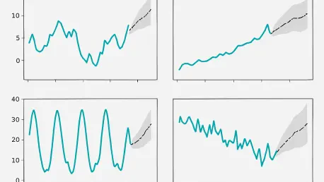
Visualization plays an indispensable role in interpreting the results of multi-model workflows, making complex data more accessible and actionable. Advanced plotting techniques in GluonTS enable the comparison of forecasts across different models, showcasing mean predictions alongside uncertainty bands to highlight confidence intervals. These visualizations also include residual distributions to analyze prediction errors and scatter plots to compare predicted versus actual values. Such detailed graphical representations provide a clear picture of how each model performs, facilitating intuitive comparisons and deeper insights into forecasting accuracy and reliability.
In addition to model-specific visualizations, performance metric comparisons are often presented through bar charts, displaying metrics like MASE and sMAPE for each estimator. This approach allows for a quick assessment of relative strengths, making it easier to identify the best-performing model at a glance. If successful forecasts are unavailable due to technical issues, a fallback option involves demonstrating concepts with synthetic data through basic plots, ensuring that key ideas are still conveyed effectively. These visualizations serve as a bridge between raw data and actionable insights, empowering users to make informed decisions based on a comprehensive understanding of model outputs and their implications for forecasting tasks.
8. Reflecting on a Robust Workflow Framework
Looking back, the journey through building multi-model workflows in GluonTS revealed a structured yet adaptable approach to time series forecasting. The process tackled data generation with synthetic series, tested various models under a unified pipeline, and delivered intuitive visual comparisons that clarified performance differences. This framework stood out for its ability to handle multiple configurations seamlessly, ensuring that even when certain dependencies were absent, the workflow remained operational through fallback mechanisms. Each step, from setup to evaluation, was executed with precision, creating a cohesive system that balanced technical complexity with practical usability.
As a final consideration, the modular design established a strong foundation for future experimentation with GluonTS, whether applied to synthetic or real-world datasets. The adaptability and robustness of this approach made it possible to scale and refine the pipeline for diverse forecasting challenges. Moving forward, exploring additional models, fine-tuning parameters, or integrating new visualization techniques could further enhance outcomes. This established framework serves as a reliable starting point, encouraging continuous learning and adaptation in the dynamic field of time series analysis, ensuring that forecasting efforts remain both innovative and grounded in solid methodology.