
Researchers transitioning from the R ecosystem to Python can leverage their existing knowledge of ggplot2 because plotnine intentionally replicates its naming conventions and architecture. This symmetry allows for a seamless shift between languages without abandoning the powerful Grammar of Graphics conceptual framework established by Leland Wilkinson. In the contemporary scientific landscape, the ability to visualize complex datasets is no longer a luxury but a fundamental requirement for transparency and analytical rigor. While libraries like Matplotlib offer granular control, they often demand verbose code that obscures the underlying logic of the data representation. Plotnine solves this problem by providing a declarative interface where visual properties are mapped directly to data variables, enabling scientists to describe what they want to see rather than how to draw every individual pixel. This efficiency is critical in 2026, as the volume of experimental data continues to grow, requiring more automated and reproducible workflows. By adopting a system that integrates natively with the pandas and Polars ecosystems, researchers can ensure their visual outputs are as robust as their statistical models, facilitating a higher standard of scholarly communication and peer-reviewed clarity across various disciplines.
The shift toward declarative plotting represents a significant evolution in data science, moving away from imperative commands that specify the exact placement of line segments or shapes on a coordinate plane. Instead, Plotnine encourages researchers to think in terms of layers, aesthetics, and scales, which aligns more closely with the mental models used during experimental design. When a researcher maps a categorical variable to a color aesthetic, they make a logical connection between the data and its visual representation. Plotnine handles the heavy lifting of generating legends, scaling axes, and ensuring that visual elements remain consistent across different subsets of the data. This high-level abstraction not only saves time but also reduces the likelihood of manual errors that can occur when hard-coding figure elements. As researchers work through iterative cycles of exploratory data analysis, the ability to rapidly change an aesthetic mapping or swap a geometric layer becomes an invaluable asset for discovering patterns that might otherwise remain hidden in raw tabular formats.
1. Environment Configuration: Detailed Procedures for System Installation and Software Dependencies
Establishing a stable environment is the first step toward generating high-quality research figures, and plotnine is designed to fit modern Python development standards. As of 2026, the package is easily accessible through the Python Package Index and Conda Forge, ensuring compatibility across various operating systems and computational setups. For most users, a standard installation via pip is sufficient, but those working in scientific research often benefit from the “extra” bundle. This extended version includes specialized libraries such as scikit-misc for advanced smoothing techniques like LOESS, and adjustText, which is essential for preventing overlapping labels in dense scatter plots. By choosing the right installation path, researchers can unlock a comprehensive suite of tools that go beyond basic plotting, providing the statistical depth required for complex biological, physical, or social science datasets. Utilizing modern environment managers like uv or pixi further streamlines this process, allowing for reproducible dependency management that is vital for long-term project viability.
Beyond the basic installation, understanding the underlying stack is helpful for troubleshooting and optimization. Plotnine is built on top of Matplotlib, which means it inherits the robust rendering capabilities and diverse backend support of the most mature visualization library in the Python ecosystem. This relationship allows researchers to use Matplotlib functions for low-level adjustments if necessary, though the declarative nature of plotnine usually makes such interventions unnecessary. Furthermore, plotnine’s reliance on NumPy and pandas ensures that data manipulation remains fast and efficient, even when dealing with millions of observations. For institutions that prioritize open-source software, the MIT License of plotnine provides the legal freedom to use and modify the library in both academic and commercial settings. This accessibility has fostered a growing community of contributors who continue to refine the package, ensuring it remains at the cutting edge of data visualization technology throughout 2026 and the years to follow.
2. Establishing a Solid Structural Foundation by Organizing Information and Implementing Effective Plot Initialization Techniques
The effectiveness of a plotnine figure depends heavily on the structure of the input data, which must be in a tidy format. In this configuration, every row represents a single observation and every column represents a unique variable, a standard that facilitates predictable mapping between data and visual aesthetics. When researchers prepare their datasets in pandas or Polars, they must ensure that categorical variables are correctly identified, as this influences how plotnine handles scales and legends. For example, if a dose-response experiment involves discrete concentrations, treating those values as strings or categorical objects rather than continuous floats prevents the library from incorrectly interpolating between them. This attention to data hygiene at the outset simplifies the plotting code significantly, as the library can automatically infer the most appropriate visual representations based on the underlying data types, thereby reducing the need for manual overrides later in the design process.
Once the data are structured, the visualization process begins with the ggplot() function, which serves as the foundation for the entire graphic. Inside this function, the aesthetic mapping (aes()) defines the primary relationships between the dataset and the visual canvas, such as identifying the x-axis, y-axis, and any color or fill groupings. A unique aspect of using plotnine in Python is the best practice of wrapping the entire multiline plot expression in parentheses. This allows researchers to chain various layers together using the plus operator without encountering the syntax errors that typically arise from Python’s whitespace sensitivity. By initializing the plot in this manner, the researcher creates a dynamic object that can be stored in a variable, modified with additional layers, or passed into custom functions. This modular approach is particularly useful for large-scale studies where the same basic plot structure must be applied across dozens of different experimental cohorts or time-series variables.
3. Geometric Layers: Incorporating Visual Shapes and Data Representations
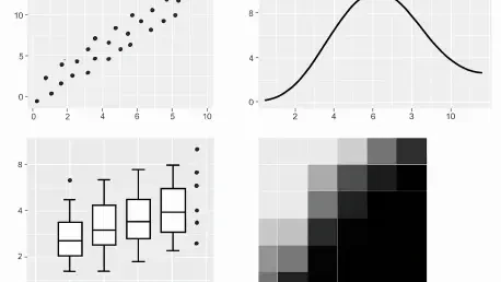
After establishing the foundation, the researcher adds geometric layers, known as geoms, to define how the data points are actually rendered on the screen. For research figures, it is common to stack multiple geometries to provide a more comprehensive view of the data distribution. For instance, combining geom_boxplot() with geom_jitter() allows the viewer to see both the summary statistics—such as the median and interquartile range—and the individual raw data points. This transparency is vital in scientific publishing, as it reveals the underlying variance and sample size that a simple bar chart or boxplot might obscure. The order in which these layers are added matters; typically, summary layers are placed first with a higher transparency or a specific alpha level, while raw data points are overlaid to highlight outliers or specific patterns. This layered approach enables the creation of complex, information-dense figures that remain legible and intellectually honest.
Beyond simple points and boxes, plotnine supports a wide array of statistical geometries that can automate complex calculations. The geom_smooth() function, for example, can fit linear models or nonlinear curves directly to the data, complete with shaded confidence intervals, without the researcher needing to perform external regression analysis. This tight integration of statistics and visualization ensures that visual trends are mathematically grounded. Furthermore, faceting functions like facet_wrap() or facet_grid() allow researchers to split a single plot into multiple subpanels based on categorical variables. This technique, often referred to as small multiples, is one of the most effective ways to compare trends across different experimental conditions, such as cell lines or treatment groups, while maintaining identical scales across all panels. By automating the creation of these panels, plotnine eliminates the tedious task of manually aligning separate images in a graphic design tool, ensuring that the final output is both accurate and professional.
4. Aesthetic Refinement: Implementing Professional Styling for Figures and Incorporating Clear, Descriptive Annotations
A raw plot, while informative, often requires significant polishing to meet the rigorous standards of academic journals. Plotnine facilitates this through its extensive theme system, which allows researchers to control every non-data element of the figure. The use of predefined themes like theme_bw() or theme_classic() is a common starting point, as these options remove the default gray backgrounds and grid lines that can distract from the data itself. Beyond these presets, the theme() function provides granular control over typography, margin sizes, and legend placement. In the context of 2026 research standards, clear and accessible design is paramount; this includes selecting high-contrast color palettes that are colorblind-friendly and ensuring that font sizes are large enough for both digital viewing and physical print. Customizing these elements ensures that the figure communicates its message effectively to a diverse audience of peers and reviewers.
Annotations and labeling serve as the final layer of clarity, transforming a data visualization into a self-contained narrative. The labs() function allows researchers to provide descriptive titles, subtitles, and captions, as well as rename the axes to include necessary units of measurement. In a research paper, a well-labeled axis like “Relative Viability (%)” is far more useful than a simple variable name like “viab_res.” Additionally, when certain data points require specific emphasis, functions like geom_text() or its more advanced counterparts can be used to add labels directly to the plot. Because plotnine is built for reproducibility, these labels are generated programmatically, meaning that if the underlying data changes, the labels will update or move accordingly. This programmatic styling ensures that the visual identity of a research project remains consistent across multiple figures, contributing to a professional and cohesive presentation in manuscripts, posters, and digital presentations.
5. Generating High-Resolution Output by Exporting Your Final Digital Images for Professional and Commercial Use
The final stage of the visualization workflow is the export process, where the digital plot is converted into a high-resolution file suitable for publication. Plotnine’s save() method is a powerful tool that leverages various Matplotlib backends to produce files in multiple formats. For manuscript submissions, vector formats such as PDF or SVG are generally preferred because they maintain infinite scalability; text and lines remain sharp regardless of how much the image is enlarged. This is particularly important for journals that require figures to be integrated into complex layouts. Alternatively, if a raster format is required, Plotnine can export PNG or TIFF files at specific resolutions, with 300 to 600 dots per inch being the standard for high-quality print. By specifying the physical dimensions in inches or centimeters directly in the save() command, researchers can ensure that the figure fits perfectly within the column widths specified by the target journal.
Choosing the right export settings also involves considering the final destination of the figure, as a high-resolution PNG might be more convenient for a conference slide deck while a vector PDF is essential for a large-format poster. Plotnine allows researchers to define the DPI and aspect ratio independently, ensuring that the visual proportions of the elements—such as point sizes and line thicknesses—scale appropriately with the physical size of the output. This level of control prevents common issues where a figure looks correct on a small laptop screen but becomes illegible when scaled up for a professional print. By automating the export process within a Python script, researchers also create a reproducible path from data to figure; any updates to laboratory findings can be reflected in the final manuscript graphics with a single click, eliminating the risk of using outdated versions of an image during the final stages of the writing process.
6. Comparison and Reliability: Troubleshooting and Visual Alternatives
Working with plotnine occasionally presents challenges, particularly for those new to the Python environment or those transitioning from more manual plotting tools. One of the most common issues is the syntax error related to the plus operator, which must be addressed by ensuring the plot code is contained within parentheses. Another frequent hurdle involves the handling of continuous versus discrete scales; when a numeric ID is used to represent a group, plotnine may attempt to apply a gradient color scale unless the researcher explicitly casts that variable as a category. Understanding these nuances is essential for maintaining a smooth workflow. For those working on headless servers or remote high-performance computing clusters, setting the Matplotlib backend to a non-interactive one like Agg is a necessary step to prevent errors related to the lack of a graphical display. These troubleshooting skills ensure that the visualization process remains robust, even in complex computational environments.
While plotnine is an exceptional tool for Grammar of Graphics enthusiasts, it exists within a diverse ecosystem of Python visualization libraries, each with its own strengths. Matplotlib remains the industry standard for low-level customization and is often used as the engine behind other libraries. Seaborn offers a higher-level interface for creating common statistical plots with less code, making it ideal for quick exploratory sessions. Altair, on the other hand, excels at creating interactive web-based visualizations using a different declarative logic. Despite these alternatives, plotnine remains the preferred choice for researchers who value the specific logic of ggplot2 and need to create complex, static figures for formal publications. By understanding the landscape of these tools, a researcher can select the most appropriate library for their specific task, whether it is a quick check of data trends or the creation of a definitive figure for a landmark study in 2026.
Advancing Scientific Reproducibility Through Visualization
The process of building professional research figures with plotnine has successfully bridged the gap between complex data analysis and high-quality visual communication. By following a structured approach—from environment setup and data cleaning to the careful layering of geometries and themes—researchers have gained the ability to produce manuscript-ready graphics that are both aesthetically pleasing and scientifically accurate. The transition from manual plotting to a declarative, grammar-based system represented a fundamental shift in how data is interpreted and shared within the scientific community. Over the past year, these workflows established a new benchmark for reproducibility, ensuring that the visual evidence supporting a hypothesis is as verifiable as the statistical tests themselves. Scientists who mastered these techniques found that their ability to communicate nuanced findings to peer reviewers and the broader public was significantly enhanced.
Looking forward, the integration of visualization tools into automated data pipelines will continue to define the standard for open science. Researchers should consider developing reusable theme templates and plotting functions that can be shared across laboratory groups to maintain visual consistency and save time. Furthermore, as the volume of high-dimensional data grows, the use of faceting and layered geometries will become even more critical for distilling complex experimental results into digestible formats. The next logical step for those proficient in plotnine is to explore the integration of these static figures into dynamic reporting tools like Quarto or Jupyter, where the code, data, and visual output coexist in a single, live document. This approach not only streamlines the publication process but also fosters a culture of transparency that is essential for the continued advancement of scientific knowledge in 2026 and beyond.